Word Embedding System
Download as PDF · 2.5 MBIntroduction
In this project, a word embedding model was developed from scratch using a self-constructed text corpus. The main objective was to implement the core algorithms without relying on external machine learning libraries. By doing this, the focus was on understanding the mathematical foundations behind distributional semantics and how these models are able to learn meaningful vector representations of words.
This work was carried out as part of my “Chosen Project”, a 7 ECTS university project supervised by Dr. Christian Steineder at Hochschule Campus Wien. The motivation for choosing this topic comes from my academic focus during my studies, where I decided to specialize in Artificial Intelligence and Machine Learning. These were the areas that quickly sparked the most curiosity and interest for me.
During lectures and especially in practical lab exercises, we often relied on existing libraries to build and experiment with machine learning models. Typically, we trained models, adjusted hyperparameters, and observed how these changes influenced metrics such as the model’s loss function. While these tools are very useful for learning how to apply machine learning in practice, they also abstract away many of the underlying mechanisms. Even though our curriculum included mathematically intensive exercises and dedicated mathematics courses in earlier semesters, most implementations still relied on high-level frameworks that hide many of the lower-level details.
For this project, I wanted to explore these mechanisms in more detail. Instead of only using existing implementations, the goal was to recreate the core components of a word embedding model myself. By implementing the mathematical operations directly and working closer to the underlying algorithms, the project aims to build a clearer understanding of how word embeddings capture semantic relationships between words and represent them as vectors in a high-dimensional space.
This article was written gradually over the duration of the project rather than being composed all at once. Because of this, different sections reflect the various stages of development and research. In the early phases, most of the time was spent reading papers and researching existing approaches. This included technical papers such as those introducing the word2vec models, as well as some linguistic literature explaining how semantic meaning emerges from words appearing together in similar contexts.
The Distributional Hypothesis
The distributional hypothesis is one of the core ideas behind modern word embeddings. It is often motivated by referring to the work of linguist Zellig Harris, who advocated a distributional methodology for studying language. The basic idea is that linguistic elements can be analyzed and categorized based on the contexts in which they appear. This idea is often summarized by a well-known statement from the British linguist J. R. Firth, written in his 1957 Synopsis of Linguistic Theory, 1930–1955: “You shall know a word by the company it keeps.”
As described by Magnus Sahlgren, a computational linguist, "Harris proposed that members of certain linguistic classes behave similarly in terms of their distribution in language". Because of this, they can be grouped together based on their distributional behavior.
For example, if we observe that two linguistic elements, w₁ and w₂, show similar distributional patterns, such as both appearing with another element w₃, we may infer that w₁ and w₂ belong to a similar linguistic category. In other words, words that occur in similar contexts tend to have related meanings.
Harris argued that language could be systematically analyzed through these distributional patterns. In his view, explanations based on distributional structure were sufficient for many linguistic analyses, without necessarily relying on additional information such as historical background or explicit semantic interpretation.
In simpler terms, the distributional hypothesis can be summarized as follows: words that have similar meanings tend to occur in similar contexts. Instead of defining meaning directly, distributional approaches infer meaning from patterns of word usage within text. In other words, meaning is derived from how words appear and interact with other words in language.
Everything in this project comes from this one idea.
Meaning
While researching this topic, this idea was quite astonishing to me. I had never really thought about how the meaning of words could be captured and represented mathematically in a meaningful way. Mathematics usually describes structures that exist in the natural world, so it initially felt surprising that human-created language could also be represented using mathematical structures that allow computers to learn relationships between words.
From a slightly more philosophical perspective, this might be explained by the fact that human language, although created and shaped by people, still emerges from natural patterns of human communication. Since language evolves through repeated structures of expression and interaction, it is not entirely surprising that these patterns can be described mathematically.
The key insight is that meaning arises from relationships between words within the language system. In distributional linguistics, two important types of relationships are commonly discussed.
1. Syntagmatic relationships
Syntagmatic relationships describe words that frequently occur together within a sequence of text. In this case, words are related because they co-occur in similar contexts.
Example: the word coffee often appears together with words such as drink, cup, morning or café.
These relationships capture combinational meaning, meaning how words are used together in natural language.
2. Paradigmatic relationships
Paradigmatic relationships describe words that can substitute for each other in a similar context. In this case, words are related because they share similar neighbors or appear in similar contexts.
Example: good news and bad news. The words good and bad can appear in the same position within the phrase.
These relationships capture similarity or category membership between words.
A distributional model therefore does not capture meaning in the way humans experience it mentally. Instead, it captures meaning as it appears in text. The resulting vector representations reflect linguistic meaning derived from patterns of word usage.
Vector Space Models of Meaning
Words as Vectors
How can we represent words, or precisely meaning of words in a way that a computer can process? One possible approach is to represent words using numbers. Word embeddings are numerical representations of words in the form of vectors. This means that each word can be represented as a list of numbers, which allows us to place words inside a mathematical vector space.
The idea of representing words and documents as vectors is not entirely new. One of the earliest influential approaches was Latent Semantic Analysis (LSA), introduced in 1990 by Deerwester et. al. In their work on information retrieval, the authors showed that patterns of word usage across documents can be represented using linear algebra. By analyzing large term-document matrices and reducing their dimensionality, LSA was able to uncover latent semantic relationships between words and texts. This idea, that meaning can emerge from statistical patterns of word usage, later became a key foundation for modern word embedding models.
For example, the word coffee could be represented by a vector that encodes how frequently it appears in certain contexts:
$$ \mathbf{v}_{\text{coffee}} = \begin{bmatrix} 8 & 5 & 6 \end{bmatrix} $$
Here, each dimension corresponds to a specific context word. For example, the dimensions could represent the contexts cup, morning, and drink. The vector therefore describes how strongly the word coffee is associated with each of these contexts.
This representation can be constructed using a word-context matrix. In this matrix, each row corresponds to a word and each column corresponds to a context feature. The entries represent how often a word appears in a particular context within a corpus:
$$ M = \begin{array}{c|ccc} & \text{cup} & \text{morning} & \text{drink} \\\hline \text{coffee} & 8 & 5 & 6 \\ \text{tea} & 7 & 4 & 6 \\ \text{book} & 0 & 1 & 0 \end{array} $$
Each row of this matrix corresponds to a vector representation of a word. For example, the vector for coffee is simply the first row of the matrix:
$$ \mathbf{v}_{\text{coffee}} = \begin{bmatrix} 8 & 5 & 6 \end{bmatrix} $$
Similarly, another word such as tea might appear in similar contexts, resulting in a vector like:
$$ \mathbf{v}_{\text{tea}} = \begin{bmatrix} 7 & 4 & 6 \end{bmatrix} $$
For better understanding, we can illustrate this for two context features in a two-dimensional space. We then consider the context features associated with cup and morning.
Example with 2 context features: $$ M = \begin{array}{c|ccc} & \text{cup} & \text{morning} \\\hline \text{coffee} & 8 & 5 \\ \text{tea} & 7 & 4 \\ \text{book} & 0 & 1 \end{array} $$
We can plot these words as points on a graph, or so called semantic feature space, where the x axis represents cup and the y axis represents morning:

As shown in the illustration, the words coffee and tea appear close to each other in the vector space. This indicates that they share similar contexts, such as cup or morning. In contrast, the word book appears further away because it does not typically occur in the same contexts.
Another way to understand this is through simple sentence completion. If we consider the sentence “In the morning I drink ____”, words such as coffee or tea fit naturally, whereas a word like book would not make sense in that context. Distributional models capture this intuition by placing words that occur in similar contexts closer together in the vector space.
Cosine Similarity
We can visually see that the words coffee and tea are close to each other, but how do we mathematically measure this? In a vector space model this means that their vectors should point in similar directions. One common way to measure this similarity is by using cosine similarity:
$$ \mathrm{sim}({v}_{w_1},{v}_{w_2}) = \cos(\theta) = \frac{\mathbf{v}_{w_1} \cdot \mathbf{v}_{w_2}} {\|\mathbf{v}_{w_1}\|\|\mathbf{v}_{w_2}\|} $$
This measures how similar two vectors are by calculating the cosine of the angle between them. It is calculated by taking the dot product of the vectors and dividing it by the product of their magnitudes. We will look at the dot product on its own in §3.3; for now, treat the \(\mathbf{v}_{w_1} \cdot \mathbf{v}_{w_2}\) in the numerator as the sum of products of matching coordinates, just as it would be written out in the formula. Because of this normalization, the measure depends only on the angle between the vectors rather than their lengths.
The value of cosine similarity lies between \(-1\) and \(+1\). A value of \(+1\) means the vectors point in the same direction (they are proportional), 0 means they are orthogonal and share no directional similarity, and \(-1\) indicates they point in exactly opposite directions. In situations where vector components cannot be negative, the possible values are restricted to the range from 0 to 1.
For example, comparing the vectors for coffee and tea:
$$ \cos(\theta) = \frac{8\cdot7 + 5\cdot4} {\sqrt{8^2 + 5^2}\sqrt{7^2 + 4^2}} \approx 0.99 $$
Since the cosine similarity is close to 1, the vectors point in a similar direction, meaning the words appear in similar contexts and are therefore semantically related.

As shown in the illustration, the similarity between two words can be interpreted as the angle \(\theta\) between their vectors. The smaller the angle between the vectors, the more similar their directions are, which indicates that the words appear in similar contexts. If the vectors point in almost the same direction, their cosine similarity approaches 1.
In the extreme case where the vectors point in exactly the same direction, the angle becomes \( \theta = 0^\circ \) and the cosine similarity is
$$ \cos(0) = 1 $$
In this way, the meaning of a word is not explicitly defined, but inferred from the contexts in which it appears. The vector representation therefore captures patterns of word usage within the corpus.
At this point one question that you might have asked is: if two vectors point in the same direction, how does that automatically mean that they are close to each other? And you are right, just because the vectors point in the same direction does not mean automatically that they are close to each other. Two vectors can have a very similar direction, but still be far apart in space. We will return to that gap in §3.4 with the Euclidean distance. First however, the dot product hiding inside the cosine formula deserves a closer look on its own.
The Dot Product
We just saw the dot product appear inside the cosine similarity formula, the \(\mathbf{v}_{w_1} \cdot \mathbf{v}_{w_2}\) in the numerator, carrying the alignment information. It deserves a section of its own, both because cosine similarity is built directly on top of it and because it will reappear in §4 when we build a training algorithm from scratch. The dot product is a small piece of arithmetic with a surprisingly large geometric meaning.
The dot product of two vectors is defined coordinate by coordinate. If \(\vec{a} = (a_1, a_2, \ldots, a_n)\) and \(\vec{b} = (b_1, b_2, \ldots, b_n)\), then
$$ \vec{a} \cdot \vec{b} \;=\; a_1 b_1 + a_2 b_2 + \cdots + a_n b_n $$
That is the algebraic definition. It is small and easy to compute. The interesting part is that the dot product has a geometric meaning hiding inside of it. The same formula from the cosine similarity can be rewritten as:
$$ \vec{a} \cdot \vec{b} \;=\; \lVert \vec{a} \rVert \, \lVert \vec{b} \rVert \, \cos\theta $$
where \(\lVert \vec{a} \rVert\) and \(\lVert \vec{b} \rVert\) are the lengths of the two vectors and \(\theta\) is the angle between them. The two definitions are equal. This is pretty basic in vector geometry, and this exact form is what makes this really useful as a similarity score. The lengths are positive numbers that measure how big the vectors are, and \(\cos\theta\) is a number between \(-1\) and \(+1\) that measures how aligned they are. Cosine similarity, as we just saw, is what you get when you divide the dot product by the lengths and keep only the alignment factor.
Three regimes
The cosine factor splits the behaviour of the dot product into three clean cases.

Two vectors that point in the same direction have a large positive dot product. Two vectors at right angles have a dot product of exactly zero, no matter how long they are. Two vectors that point in opposite directions have a large negative dot product. Everything in between is a smooth interpolation: as you rotate one vector away from another, the dot product slides continuously from its positive maximum down through zero and on to its negative minimum.

Cosine vs. raw dot product
Cosine similarity and the dot product are not really two independent quantities, they are two views of the same algebraic object. Here is the dot product again:
$$ \vec{a} \cdot \vec{b} \;=\; \lVert \vec{a} \rVert \, \lVert \vec{b} \rVert \, \cos\theta $$
Cosine similarity is exactly the \(\cos\theta\) factor sitting in that formula, isolated by dividing both sides by the magnitudes:
$$ \cos\theta \;=\; \frac{\vec{a} \cdot \vec{b}}{\lVert \vec{a} \rVert \, \lVert \vec{b} \rVert} $$
So the dot product literally contains the cosine similarity, multiplied by the two magnitudes. Cosine strips the magnitudes off and keeps only the direction part. The dot product keeps both pieces: alignment and the lengths of the vectors involved. Whenever we use one of them, we are choosing whether or not to keep the magnitude information that the other one would either preserve or throw away. This is usually always the better and more used measurement.
One more thing worth knowing: the dot product is not a measure of distance. How far apart two vectors are is a different question, answered by Euclidean distance in §3.4. The dot product is \(\lVert \vec{a} \rVert \, \lVert \vec{b} \rVert \, \cos\theta\) and it mixes direction and magnitude (the length of the vector arrow), but neither of those is distance.
Concrete numbers make this understand better. Compare two pairs of vectors. First pair, both pointing right along the \(x\)-axis:
$$ \vec{u} = (10, 0), \qquad \vec{v} = (5, 0) $$
These vectors are \(5\) units apart in actual distance. Their three measurements:
$$ \begin{aligned} \vec{u} \cdot \vec{v} \;&=\; 10 \cdot 5 + 0 \cdot 0 \;=\; 50 \\[4pt] \cos(\theta) \;&=\; 1.0 \quad \text{(perfectly aligned)} \\[4pt] \text{Euclidean distance} \;&=\; 5 \end{aligned} $$

Second pair, again both pointing right but with much smaller vectors that are very close to each other in space:
$$ \vec{u} = (1, 0), \qquad \vec{v} = (0.95, 0.05) $$
$$ \begin{aligned} \vec{u} \cdot \vec{v} \;&=\; 1 \cdot 0.95 + 0 \cdot 0.05 \;=\; 0.95 \\[4pt] \cos(\theta) \;&\approx\; 1.0 \quad \text{(also nearly aligned)} \\[4pt] \text{Euclidean distance} \;&\approx\; 0.07 \end{aligned} $$

The first pair is further apart in distance (\(5\) vs \(0.07\)) but has a much higher dot product (\(50\) vs \(0.95\)). The dot product went up because the vectors got longer, not because they got closer. Distance and dot product are independent.
So three different measurements live in this neighbourhood, and they answer three different questions:
Cosine similarity answers do these point the same way? This means it is length-blind and it measures the range as \(-1\) to \(+1\).
Dot product answers how strongly aligned, weighted by how big the vectors are? This means it is length-aware and the range can be any real number.
Euclidean distance answers how far apart in space are they? Direction-blind in the sense that only the gap between the vector tips matters. Range can be \(0\) to \(\infty\).
For our project: Euclidean distance
While researching later, I was confused as to why most of the modern word embedding systems use the dot product instead of the Euclidean distance. I mean, the Euclidean distance literally expresses how far apart two vectors are. Wouldn't that be the more intuitive measurement to drive a learning algorithm with?
After some thinking, I came around to the answer: both of them work. For the algorithm we are building in this project, Euclidean distance is the more natural choice, and that is the route this project will take. We will follow a direct approach, where close vectors will be trained to become even closer with semantically similar words, so the euclidean distance will be a better fit.
It is worth noting up front that all three of the measurements introduced in this section cosine similarity, the dot product, and Euclidean distance can be used to drive a learning algorithm.
Cosine similarity and the dot product do not disappear though. They remain useful for comparing trained vectors after the fact. Questions like "is king closer to queen or to breakfast?" can be answered with either, and we will reach for them for exactly that once the algorithm has finished training.
With cosine similarity and the dot product now on the table as similarity tools that we can use it is time to introduce another one, which is the Euclidean distance. This will also later take the centre stage as the algorithm's training primitive.
Euclidean Distance
While cosine similarity measures the angle between two vectors, Euclidean distance measures the straight-line distance between them. In two dimensions, this is simply the usual distance formula known from mathematics.
$$ d(\mathbf{v}_{w_1}, \mathbf{v}_{w_2}) = \|\mathbf{v}_{w_1} - \mathbf{v}_{w_2}\| = \sqrt{\sum_{i=1}^{n}(v_{w_1,i} - v_{w_2,i})^2} $$
For the vectors of coffee and tea:
$$ \mathbf{v}_{\text{coffee}} = \begin{bmatrix} 8 & 5 \end{bmatrix} $$
$$ \mathbf{v}_{\text{tea}} = \begin{bmatrix} 7 & 4 \end{bmatrix} $$
we obtain:
$$ d(\mathbf{v}_{\text{coffee}}, \mathbf{v}_{\text{tea}}) = \sqrt{(8-7)^2 + (5-4)^2} = \sqrt{2} \approx 1.41 $$

This means that the two vectors are geometrically close to one another. As we already saw inside the example previously with Pair A \(\vec{u} = (10, 0)\) and \(\vec{v} = (5, 0)\), Euclidean distance and cosine similarity do not capture the same property. Two vectors can point the almost exact same direction, which would result the cosine similarity to be close to \(1\), while still being far apart in Euclidean distance if one is much longer than the other. Direction and distance are independent quantities.
This distinction matters for choosing what to use for comparing similarities. Cosine similarity is the standard choice for comparing trained word vectors after the fact, when we want to ask things like "is king closer to queen or to breakfast?" then the question is purely about direction, and cosine's fixed range of \(-1\) to \(+1\) makes the answer really easy to calculate and see. Euclidean distance on the other hand is what our training algorithm in will actually be optimising.
The same idea also applies in higher dimensions. Real word embeddings usually live in spaces with dozens or hundreds of dimensions, even though they are often illustrated in two-dimensional diagrams for simplicity. The formula stays exactly the same; you just keep adding squared coordinate-differences under the root, and the geometry with the algorithm we will build on top of it. Nothing changes.
Dimensionality and Learned Embeddings
So far the vectors in our examples have had only two or three dimensions, which is convenient for drawing pictures. A natural question is: who actually decides how many dimensions a word vector has? The short answer is that it depends on the type of model. In classical word-context matrices, the corpus decides. In modern models as word2vec, we decide.
We will write \(d\) for the chosen number of dimensions and represent each word \(w\) as a vector
$$ \mathbf{v}_w \in \mathbb{R}^d $$
Classical models. In word-context matrices, every column is a context word, and the vector for a word is just the row that records how often it appears next to each context. So if the corpus contains \(|C|\) different context words, the vectors automatically end up with \(d = |C|\) dimensions. A larger vocabulary means longer vectors, whether we want them or not.
Modern models. Word2vec and similar models do not build this matrix at all. Instead, \(d\) is picked in advance as a hyperparameter (commonly something like \(d = 300\)) and the model learns the actual numbers inside each vector during training. Formally, the model learns a mapping
$$ f : V \rightarrow \mathbb{R}^{d} $$
from the vocabulary \(V\) to vectors of length \(d\), adjusting the values so that words appearing in similar contexts end up close to each other in the resulting space.
How big should \(d\) be? More dimensions give the model more room to capture subtle patterns, but they also cost more memory and training time. In their experiments on a large Google News corpus, Mikolov et al. observed that “after some point, adding more dimensions or adding more training data provides diminishing improvements.” Pennington et al. similarly report that values between 100 and 300 usually offer a good balance between expressiveness and cost. The two factors also need to grow together: large vector spaces are only useful with enough data to fill them with meaningful patterns.
Before imagining 300 dimensions, it helps to push our earlier 2D example one step further. Here is the same coffee/tea/book vocabulary with a third context feature added, plus one new word breakfast.
Example with 3 context features: $$ M = \begin{array}{c|ccc} & \text{cup} & \text{morning} & \text{drink} \\\hline \text{coffee} & 8 & 5 & 6 \\ \text{tea} & 7 & 4 & 6 \\ \text{book} & 0 & 1 & 0 \\ \text{breakfast} & 1 & 9 & 1 \end{array} $$

In the illustration above, these vectors are visualized as points in a three-dimensional semantic space. Each axis corresponds to one context feature (cup, morning, or drink), and the coordinates of each point are taken directly from the matrix.
As explained, models often use hundreds or thousands more context features. This results in a representation with thousands of dimensions, making further dimensional visualization impossible. However, the same geometric intuition still applies.
Vector Arithmetic
Interestingly enough:
Mikolov et al. demonstrated that semantic relationships between words can sometimes be captured using simple vector arithmetic :
$$ \mathrm{king} - \mathrm{man} + \mathrm{woman} \approx \mathrm{queen} $$
The vector difference between king and man captures part of the relationship between these two words. In this case, something related to gender and social role. If we subtract the vector man and then add the vector for woman, we move inside the vector space.
Shockingly, or not, the resulting vector often points very close to the position of the word queen. This shows that the embedding space has learned meaningful relationships between words purely from patterns of word usage in text.
This idea is worth looking at more carefully, because it shows that simple vector addition and subtraction can express something close to analogical reasoning. An analogy expresses a relationship between concepts. The classic example is "man is to king as woman is to ____". To find the missing word, we first describe the relationship between man and king as a vector, and then apply that same relationship to woman.
Suppose that after training the model has assigned the following three-dimensional vectors:
$$ \begin{aligned} \mathbf{v}_{\text{king}} &= [\,1,\ 8,\ 8\,] \\ \mathbf{v}_{\text{man}} &= [\,1,\ 7,\ 0\,] \\ \mathbf{v}_{\text{woman}} &= [\,9,\ 7,\ 0\,] \\ \mathbf{v}_{\text{queen}} &= [\,9,\ 7,\ 8\,] \end{aligned} $$
We can try sutracting the vector of man with the vector of king:
$$ \mathbf{v}_{\text{king}} - \mathbf{v}_{\text{man}} = [\,1-1,\ 8-7,\ 8-0\,] = [\,0,\ 1,\ 8\,] $$
This gives us a vector of \([0,1,8]\). This difference vector captures whatever distinguishes king from man in the embedding space. If we experiment a bit further and try adding the vector of woman we shift the vector and get the following:
$$ \mathbf{v}_{\text{woman}} + (\mathbf{v}_{\text{king}} - \mathbf{v}_{\text{man}}) = [\,9+0,\ 7+1,\ 0+8\,] = [\,9,\ 8,\ 8\,] $$
The resulting vector \([9, 8, 8]\) does not exactly match any word in the vocabulary, but the closest word vector turns out to be queen at \([9, 7, 8]\). The full calculation can be summarised in a small table:
$$ \begin{array}{l|ccc} & \text{dim 1} & \text{dim 2} & \text{dim 3} \\\hline \text{king} & 1 & 8 & 8 \\ \text{man} & 1 & 7 & 0 \\ \text{king} - \text{man} & 0 & 1 & 8 \\ \text{woman} & 9 & 7 & 0 \\ \text{king} - \text{man} + \text{woman} & 9 & 8 & 8 \\ \text{queen} & 9 & 7 & 8 \end{array} $$
To find the answer to the analogy, we look for the word whose vector lies closest to the computed result, typically using the cosine similarity introduced in section 3.2. In this example, queen is the nearest neighbour, which matches our intuitive answer.
The same idea generalises to many other relationships. For instance, the difference between the vectors of king and kingdom captures something like the relation between a ruler and the place they rule, while the difference between coffee and tea in the earlier examples points roughly along the dimension that distinguishes the two drinks while leaving their shared contexts (cup, morning, drink) almost unchanged. What is remarkable is that nobody explicitly told the model about gender, royalty, or drinkware. These relationships emerge purely from the contexts in which the words appear in the corpus, and they end up encoded as consistent geometric directions in the vector space.
All of these ideas form the foundation of modern word embedding models. Instead of manually constructing large word-context matrices, ideally an algorithm should learn these vector representations automatically from large amounts of text. The training process adjusts the vectors so that words appearing in similar contexts become closer together in the vector space.
Implementation
Corpus and Preprocessing
Now enough about theory, let us implement these systems from scratch. The first practical step in this project was the construction and preparation of a suitable text corpus. A corpus that repeatedly places related words in similar contexts gives the model the necessary information to infer meaningful similarities. Conversely, a corpus that is too small, too noisy, or too inconsistent makes it much harder for the model to learn stable relationships.
For this reason, the corpus used in this project was not chosen randomly. Instead, it was self-written so that several semantic groups would appear repeatedly in overlapping contexts. Examples include words related to drinks such as coffee and tea, royal terms such as king and queen, animals such as dog and cat, vehicles such as car, bus, and train, and academic terms such as student, teacher, book, and library. The purpose of this design was to create a corpus in which meaningful distributional structure is visible even on a relatively small scale. This makes it possible to test whether the implementation is able to recover these relationships from text alone.
Everything referenced here can be found inside the GitHub Repository. Furthermore, here is the corpus as a text file.
Before the corpus can be used for training, it first had to be preprocessed. Raw text often contains many elements that are not directly useful for an initial implementation of a word embedding model, such as inconsistent capitalization, punctuation marks, and formatting differences. Since corpora are typically collected from sources such as textbooks, articles, or other written materials, they usually require some cleaning before they can be processed in a consistent and reliable way.
First, we want to normalise the text. All text was converted to lowercase so that words such as King and king would be treated as the same vocabulary item. This reduces sparsity in the data and prevents the model from learning separate vectors for words that differ only in capitalization. In addition, most punctuation marks were removed. For a first implementation, punctuation does not contribute much to the semantic patterns of interest, while keeping it would unnecessarily increase the vocabulary and complicate the representation.
def normalize_text(text):
                text = text.lower()
                text = re.sub(r"[^a-z.!?\s]", " ", text)
                text = re.sub(r"\s+", " ", text)
                return text.strip()
After normalization, the text is split into sentences. This step is important because context windows should normally be restricted to individual sentences. If sentence boundaries are ignored, the model may incorrectly treat the last word of one sentence and the first word of the next sentence as meaningful neighbors, even though they are unrelated in the original text.
After that each sentence is tokenized, meaning that it was split into individual word tokens. This was implemented in a very simple way by splitting sentences at whitespace after normalization. For large-scale industrial systems, more advanced tokenization strategies are often necessary, especially for handling punctuation, contractions, or languages with more complex morphology. However, for the purposes of this project, a simple whitespace-based tokenizer was sufficient and had the advantage of keeping the implementation transparent and easy to inspect.
    # Split the text into sentences
    def split_sentences(text):
        sentences = re.split(r"[.!?]+", text)
        return [sentence.strip() for sentence in sentences if sentence.strip()]

    # Split one sentence into words
    def tokenize(sentence):
        return sentence.split()
Vocabulary Construction
Once the corpus had been tokenized, the next step was to construct the vocabulary. Each token (word) that we split from the sentences in the vocabulary can be assigned a unique integer identifier. You can think of it as a map. In a sense, we are creating a look-up table that allows us to easily convert from words to indices, and indices to words. This table can be used in two directions: from words to indices, and from indices back to words.
A simplified example:
Suppose the sentence:
$$ \text{the king rules the kingdom} $$
appears in the corpus. After tokenization, it becomes the sequence
$$ [\text{the}, \text{king}, \text{rules}, \text{the}, \text{kingdom}] $$
If the vocabulary assigns the identifiers
$$ \begin{aligned} \text{the} &\mapsto 0, & \text{rules} &\mapsto 2, \\ \text{king} &\mapsto 1, & \text{kingdom} &\mapsto 3 \end{aligned} $$
then the sentence can be represented numerically as
$$ [0,1,2,0,3]. $$
This transformation is really important because it turns raw language into a machine-readable form.
    # Build a vocabulary by assigning each word a number
    def build_vocab(tokenized_sentences):
        word_to_id = {}
        id_to_word = {}
        current_id = 0

        for sentence in tokenized_sentences:
            for word in sentence:
                if word not in word_to_id:
                    word_to_id[word] = current_id
                    id_to_word[current_id] = word
                    current_id += 1

        return word_to_id, id_to_word
The vocabulary-building step only creates a mapping between words and integer IDs. The corpus is still stored as words at this point. In the next step, this mapping is applied to every tokenized sentence, so that each word is replaced by its corresponding ID. This produces the encoded sentences that can later be used as input for training.
After this step, the entire corpus is transformed into an array of numbers, a so called numerical representation. Each word is replaced by the integer that was previously assigned to it in the lookup table (the vocabulary). As a result, the corpus is no longer stored as words, but as sentences made up of numbers, where each number uniquely refers to one word.
The following function does that for us:
# Turn words into numbers
    def encode_sentences(tokenized_sentences, word_to_id):
        encoded_sentences = []

        for sentence in tokenized_sentences:
            encoded_sentence = []
            for word in sentence:
                encoded_sentence.append(word_to_id[word])
            encoded_sentences.append(encoded_sentence)

        return encoded_sentences
Consider the two sentences
$$ \text{The king rules the kingdom.} $$
$$ \text{The queen does not rule the kingdom.} $$
After normalization and sentence splitting, they become
$$ [\text{the},\ \text{king},\ \text{rules},\ \text{the},\ \text{kingdom}] $$
$$ [\text{the},\ \text{queen},\ \text{does},\ \text{not},\ \text{rule},\ \text{the},\ \text{kingdom}] $$
Suppose the vocabulary assigns the following IDs:
$$ \begin{aligned} \text{the} &\mapsto 0, & \text{queen} &\mapsto 4, \\ \text{king} &\mapsto 1, & \text{does} &\mapsto 5, \\ \text{rules} &\mapsto 2, & \text{not} &\mapsto 6, \\ \text{kingdom} &\mapsto 3, & \text{rule} &\mapsto 7 \end{aligned} $$
Then the encoded sentences are
$$ [0,1,2,0,3] $$
$$ [0,4,5,6,7,0,3] $$
So the numerical representation of the full input is
$$ [[0,1,2,0,3],\ [0,4,5,6,7,0,3]] $$
We can print these out inside our python code to visualise it step by step:
    with open("corpus.txt") as file:
            text = file.read()

    clean_text = normalize_text(text)
    print("Cleaned text (characters): ")
    print(clean_text[:64])

    sentences = split_sentences(clean_text)
    print("\nSentences: ")
    print(sentences[:2])

    tokenized_sentences = []
    for sentence in sentences:
        tokenized_sentences.append(tokenize(sentence))
    print("\nTokenized sentences: ")
    print(tokenized_sentences[:2])

    word_to_id, id_to_word = build_vocab(tokenized_sentences)
    print("\nWord to ID: ")
    print(list(word_to_id.items())[:10])

    print("\nEncoding the whole sentence: ")
    encoded_sentences = encode_sentences(tokenized_sentences, word_to_id)
    print(encoded_sentences[:2])
The following video walks through the entire preprocessing and vocabulary-building pipeline for a single sentence, from the raw text all the way to the final encoded representation.
Preprocessing and vocabulary-building pipeline for a single sentence.
Context Window and Training Data
Having the sentences in encoded form still does not indicate what the model is supposed to learn. Once the corpus has been preprocessed and transformed into encoded sentences, the next step is to construct the actual training data used for computation. You might already think that the encoded sentences are the data, which they are, but not yet in the exact form that captures local word relationships.
As explained in section 2 Distributional Hypothesis and 3 Vector Space Models, word embedding models do not learn directly from whole sentences at once, even when encoded as numbers. Instead, they learn from local word-context relationships inside a small window around each target word.
So we need somehow now a way to compare every encoded number inside the sentences, to their neighbors.
This local neighborhood is called the context window. If a window size of \(m\) is chosen, then for each word in a sentence, the model considers the words that occur within \(m\) positions to the left and right as its context.
Example:
Consider the encoded sentence
$$ [0,1,2,0,3] $$
which corresponds to
$$ [\text{the}, \text{king}, \text{rules}, \text{the}, \text{kingdom}]. $$
If the word king with \(id\) = \(1\) is chosen as the center word and the context window size is \(m\) = \(1\), then its context consists of the neighboring words
$$ [0,2]. $$
This produces the training pairs
$$ (1,0),\ (1,2). $$
Below a more clear illustration:

Repeating this process for every word in every sentence transforms the encoded corpus into a set of center-context pairs. These pairs form the actual training data from which the embedding model learns.
Example with a larger context window:
Consider the sentence
$$ [\text{in},\ \text{the},\ \text{morning},\ \text{i},\ \text{drink},\ \text{coffee}] $$
and suppose it is encoded as
$$ [4,0,5,6,7,8]. $$
If the word drink with \(id = 7\) is chosen as the center word and the context window size is \(m = 2\), then we look up to two positions to the left and two positions to the right of the center word.
In this case, the neighboring words are
$$ [5,6,8] $$
which correspond to
$$ [\text{morning},\ \text{i},\ \text{coffee}]. $$
This produces the training pairs
$$ (7,5),\ (7,6),\ (7,8). $$
In word form, these pairs are
$$ (\text{drink},\ \text{morning}), (\text{drink},\ \text{i}), \\ (\text{drink},\ \text{coffee}). $$
A larger context window therefore allows the model to observe a broader neighborhood around the center word. Instead of learning only from the immediately adjacent words, it can also incorporate words that are slightly farther away in the sentence.
In practice, the size of the context window is a hyperparameter of the model. Smaller windows often capture more local and syntactic relationships, while larger windows capture broader topical information. For the relatively small and structured corpus used in this project, a window size of \(m = 2\) provides a reasonable balance between capturing meaningful context and avoiding excessive noise.
These center-context pairs can also be understood in terms of a co-occurrence matrix. Such a matrix records how often a word appears near another word inside the chosen context window. Each row represents a center word, each column represents a context word, and each entry contains the number of times that this combination occurs in the corpus.
Simplified example:
Suppose the vocabulary contains only the words
$$ \{\text{drink},\ \text{coffee},\ \text{morning},\ \text{i}\}. $$
Then a possible co-occurrence matrix could look like
$$ M = \begin{array}{c|cccc} & \text{drink} & \text{coffee} & \text{morning} & \text{i} \\\hline \text{drink} & 0 & 1 & 1 & 1 \\ \text{coffee} & 1 & 0 & 0 & 0 \\ \text{morning} & 1 & 0 & 0 & 0 \\ \text{i} & 1 & 0 & 0 & 0 \end{array} $$
In this example, the row for drink shows that the word drink occurred near coffee, morning, and i. The matrix therefore summarizes local contextual information across the corpus in a structured numerical form.
A larger context window does not automatically produce a higher-dimensional matrix. The size of the co-occurrence matrix is usually determined by the vocabulary size. If the vocabulary contains \( |V| \) words, then the matrix has the size
$$ |V| \times |V|. $$
Increasing the context window size \(m\) changes how many neighboring words are counted, but it does not change the number of rows or columns. Instead, it changes the values inside the matrix, because more words are considered part of the context.
In other words, a larger context window usually makes the matrix denser, not larger. The dimensionality of the learned word vectors is a separate design choice and is controlled by the embedding dimension \(d\), which is also a hyperparameter, not by the window size \(m\).
To create such pairings we can use the following function:
class TrainingDataGenerator:
    def generate_pairs(self, encoded_sentences, window_size=1):
        pairs = []

        for sentence in encoded_sentences:
            for i in range(len(sentence)):
                center_word = sentence[i]

                start = max(0, i - window_size)
                end = min(len(sentence), i + window_size + 1)

                for j in range(start, end):
                    if i != j:
                        context_word = sentence[j]
                        pairs.append((center_word, context_word))

        return pairs
Using the corpus constructed for this project, the function produces training pairs such as the following:
First 10 training pairs:
          (0, 1) -> the king
          (1, 0) -> king the
          (1, 2) -> king rules
          (2, 1) -> rules king
          (2, 0) -> rules the
          (0, 2) -> the rules
          (0, 3) -> the kingdom
          (3, 0) -> kingdom the
          (0, 4) -> the queen
          (4, 0) -> queen the
One thing that might look surprising in the output is that both (0, 1) -> the king
and (1, 0) -> king the appear. These are not duplicate mistakes, but two different
training observations. The pair \((0,1)\) means that king appeared in the context
of the, while \((1,0)\) means that the appeared in the context
of king. Since the function treats each word in turn as the center word, the same
two neighboring words show up again with their roles reversed. In this way, the algorithm systematically
transforms the encoded corpus into a collection of local word-context relationships.
The following visual explanation showcases this process of pair-building:
Pair-building process from encoded sentences.
The output shown above is therefore the direct result of sliding a small context window through the corpus sentence by sentence. Each line records one such local observation. Across the entire corpus, these observations form the training data from which the embedding model later learns which words tend to occur in similar contexts.
Creating Word Vectors
Once the training pairs have been generated, the next step is initialise the vectors and to define how the model learns from them. Up to this point, the corpus has only been transformed into a numerical form and decomposed into local word-context observations. The embedding model now uses these observations to learn a vector representation for each word in the vocabulary.
The central idea is that every word \(w \in V\) is assigned a vector
$$ \mathbf{v}_w \in \mathbb{R}^d $$
where \(d\) is the embedding dimension chosen in advance.
import random

class EmbeddingModel:
    def __init__(self, vocab_size, embedding_dim=5):
        self.vocab_size = vocab_size
        self.embedding_dim = embedding_dim

        self.embeddings = []
        for _ in range(vocab_size):
            vector = []
            for _ in range(embedding_dim):
                vector.append(random.uniform(-0.5, 0.5))
            self.embeddings.append(vector)

    def get_vector(self, word_id):
        return self.embeddings[word_id]
At the beginning, these vectors are initialized with small random values between \( [-0.5, 0.5] \). They do not yet contain meaningful semantic information, we just want them initialised. During training, the vectors are gradually adjusted so that words appearing in similar contexts become closer together in the embedding space.
We can afterwards verify this 5 dimensional random assigned vector:
# Part 3 - Embedding model
    model = EmbeddingModel(vocab_size=len(word_to_id), embedding_dim=5)

    print("Vector for 'king':")
    print(model.get_vector(word_to_id["king"]))

    print("\nVector for 'queen':")
    print(model.get_vector(word_to_id["queen"]))
\[ \text{Vector for "king"} = \begin{bmatrix} 0.479 \\ 0.187 \\ 0.017 \\ -0.457 \\ -0.003 \end{bmatrix} \]
The function only assigns vectors to already mapped words. When trying to get the vector of a word that is not in the vocabulary we get an error.
Now that we have the vectors, we need to adjust them accordingly. The word-context pairs generated in the previous step provide the learning signal for this adjustment process. If a word repeatedly appears with certain neighboring words, then its vector should become similar to the vectors of other words that occur in comparable contexts. In this way, semantic structure emerges from repeated contextual patterns in the corpus.
Simplified Learning from Pairs
The simplest possible idea for learning from these pairs is this: every time we observe two words as a pair, we nudge their vectors a tiny step closer together. If king and rules appear next to each other, we pull the vector of king slightly toward the vector of rules, and vice versa. After repeating this process across the entire corpus, words that share many context partners end up clustered in the same region of the vector space, while unrelated words drift apart.
Mathematically, for each dimension \(i\) of the embedding, the update rule for a center-context pair is
$$ \begin{aligned} v_{\text{center},i} &\leftarrow v_{\text{center},i} + \eta \cdot (v_{\text{context},i} - v_{\text{center},i}) \\ v_{\text{context},i} &\leftarrow v_{\text{context},i} + \eta \cdot (v_{\text{center},i} - v_{\text{context},i}) \end{aligned} $$
where \(\eta\) is the learning rate. The learning rate controls how strongly the vectors are adjusted after each observed pair. A small value means gentle, gradual updates, while a larger value means the vectors move more aggressively after every training run (epoch).
An important detail of this update rule is that both equations use the pre-update
values of the two vectors. This means that the new value of \(v_{\text{center},i}\) is computed from the
old \(v_{\text{context},i}\), and the new value of \(v_{\text{context},i}\) is computed from
the old \(v_{\text{center},i}\). The two updates therefore happen at the same time
rather than sequentially, and this is exactly what we want.
If we instead updated the center vector first and then used its already
modified value when updating the context vector, the update would no longer be symmetric and the
two vectors would not move toward each other by the same amount. This is why we first store the current values as center_value and
context_value before writing any new values back into the embedding matrix.
In practical terms, this means that the next stage of the implementation needs a data
structure for storing word vectors, an initialization strategy, and a rule for updating these
vectors whenever a training pair is observed. To achieve this we can implement a
train_on_pair function that takes a single center-context pair and applies the
update rule above. For this project the learning rate is set to \(\eta = 0.1\).
import random

class EmbeddingModel:
    def __init__(self, vocab_size, embedding_dim=5):
        self.vocab_size = vocab_size
        self.embedding_dim = embedding_dim

        self.embeddings = []
        for _ in range(vocab_size):
            vector = []
            for _ in range(embedding_dim):
                vector.append(random.uniform(-0.5, 0.5))
            self.embeddings.append(vector)

    def get_vector(self, word_id):
        return self.embeddings[word_id]

    def train_on_pair(self, center_word, context_word, learning_rate=0.1):
        center_vector = self.embeddings[center_word]
        context_vector = self.embeddings[context_word]

        for i in range(self.embedding_dim):
            center_value = center_vector[i]
            context_value = context_vector[i]

            center_vector[i] = center_value + learning_rate * (context_value - center_value)
            context_vector[i] = context_value + learning_rate * (center_value - context_value)
More precisely, for each dimension \(i\) the function first takes a snapshot of the current
values of the center and context vectors (center_value and context_value)
and only then uses these snapshots to compute the new values of both vectors.
Repeating this process over many observed pairs gradually shapes the embedding space according
to the contextual structure of the corpus.
Example:
In a training pair, the center vector is the vector of the current target word, while the context vector is the vector of one neighboring word inside the chosen context window. For example, if the pair is
\[ (\text{king},\ \text{rules}) \]
then the vector of king is treated as the center vector and the vector of rules is treated as the context vector. The update step then compares these two vectors coordinate by coordinate and moves them slightly toward one another.
The vectors of the words are initiated randomly at the beginning, so suppose the vectors are:
\[ \mathbf{v}_{\text{king}} = \begin{bmatrix} 0.479 \\ 0.187 \\ 0.017 \\ -0.457 \\ -0.003 \end{bmatrix} \qquad \mathbf{v}_{\text{rules}} = \begin{bmatrix} 0.120 \\ -0.050 \\ 0.210 \\ -0.300 \\ 0.400 \end{bmatrix} \]
If the learning rate is \(\eta = 0.1\) then the vectors are updated coordinate by coordinate so that the corresponding values move slightly towards one another. For the first coordinate, the value of the center vector is \(0.479\) and the value of the context vector is \(0.120\). Using the update rule, we obtain
$$ v_{\text{king,1}} \leftarrow 0.479 + 0.1(0.120 - 0.479) = 0.4431 $$
$$ v_{\text{rules,1}} \leftarrow 0.120 + 0.1(0.479 - 0.120) = 0.1559 $$
The two values are therefore closer after the update than before. The same idea is then applied to the second coordinate, the third coordinate, and so on until all five dimensions have been updated. In this way, the vector of king and the vector of rules move slightly closer together in the embedding space whenever this pair is observed during training.
This may sound really good on paper, but when we run the algorithm over multiple epochs, an issue becomes apparent. The vectors move closer and closer together until they eventually collapse into the same region of space.
The reason is that our simplified approach only pulls. Every observed pair results in two vectors moving slightly closer, but there is no mechanism to push unrelated words apart. Attraction is the only force acting on the system, so given enough epochs the vectors have nowhere to settle except on top of one another.
It is important to note that this simplified training algorithm is inspired by the central idea behind models such as word2vec, where words that appear in similar contexts should obtain similar vector representations. However, it captures only one half of that mechanism. The other half that we need to implement is a repulsion. So words who are not neighbours should be pushed away.
In the actual word2vec model, learning is formulated as an optimization problem with both attraction and repulsion. For every real (center, context) pair such as (king, rules), the model also randomly samples a few words that did not appear near the center word, for example (king, coffee). The model is then trained to give the real pair a high compatibility score and the sampled pairs a low score. This push-and-pull mechanism, called negative sampling, is what allows word2vec to produce sharp, well-separated word representations rather than a single fuzzy cluster.
Running the Direct Approach
We can run the direct approach over a certain amount of epochs:
    # Part 4 - Simplified Learning from pairs
    EPOCHS = 100
    LEARNING_RATE = 0.01

    print(f"\nTraining for {EPOCHS} epochs (learning rate = {LEARNING_RATE})...")
    for epoch in range(1, EPOCHS + 1):
        random.shuffle(pairs)
        for center, context in pairs:
            model.train_on_pair(center, context, learning_rate=LEARNING_RATE)
        if epoch % 10 == 0:
            print(f"  Epoch {epoch}/{EPOCHS} done")

    print("\nVector for 'king' after training:")
    print(model.get_vector(word_to_id["king"]))

    print("\nVector for 'queen' after training:")
    print(model.get_vector(word_to_id["queen"]))
We train the model on the full corpus for 200 epochs. In the example above, the vectors for king and queen are shown both before training and after the final epoch. Because this is a bit hard to visualise, we can get the each words vector after every run and use the Matplot library to plot how all vectors change over time, making the progression easier to visualise.
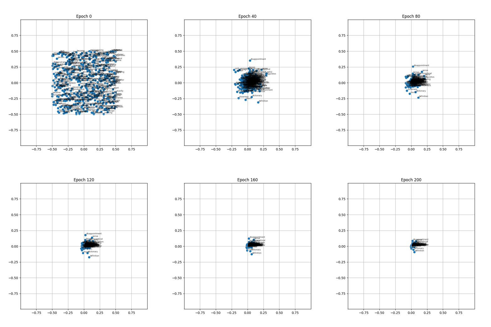
At epoch 0 the vectors sit where the random initialisation placed them, spread roughly evenly across the plane. Within the first few epochs the whole mass begins to drift inward. By a few dozen epochs the labels are densely stacked on top of each other near the center, and by the time the animation finishes every vector occupies almost exactly the same point.
I have ported the preprocessing pipeline and the train_on_pair function into JavaScript and prepared a simulation inside the browser. It
uses a small built-in corpus that covers most of the same semantic topics of the project corpus
(royalty, drinks, academia, pets, vehicles) and exposes the hyperparameters: the learning rate, the window size, and the embedding dimension.
Inside one epoch, the full list of (center, context) pairs is shuffled and then every
pair is fed through the direct-approach rule.
The scatter plot on the left shows the current position of every word vector. When \(d = 2\), what you see is the full embedding space. When \(d > 2\), only the first two coordinates are drawn and the viewport still spans \([-0.6, 0.6]\) on both axes, so it is honest about the fact that you are looking at a slice. The metrics panel on the right operates on the full vector regardless of \(d\), so the numbers it reports are not affected by the projection.
Two metrics are tracked over time. The blue curve is the mean pairwise Euclidean distance between all pairs of word vectors. At initialisation it is a random positive number set by the random draw in \([-0.5, 0.5]\). During training it should only decrease. The gray curve is the mean vector norm, whic means it is the average length of a word vector. Together they summarise how much the embedding space is shrinking and how far from the origin its centre of mass sits.
What you can and cannot see in the simulator
Running the simulator at a small learning rate, what you can see most clearly is the effect of initialisation. When two related words happen to start near each other, they stay near each other while the whole cloud drifts inward, and this looks like a tight semantic cluster. When they start far apart, attraction does pull them together over time, but the global collapse overwrites them before any structure becomes visually distinguishable. The figure below is a favourable run in which the royalty and beverage groups happen to initialise in close proximity to their respective partners, a controlled demonstration rather than a typical outcome.

We can see the distributional semantics here really nicely. The words king and queen never appear in the same sentence of the corpus, they are not a (center, context) pair in any epoch, so the attraction rule never directly pulls them together. But they lie close to each other. What brings them close is that they share context words like rules and kingdom: each is pulled toward rules, each is pulled toward kingdom, and over time this shared relationship leaves them near each other. The similarity is indirect, it is developed by the contexts they have in common rather than by direct co-occurrence.
Another observaion is harder to see but worth naming: in the first few dozen epochs, related words co-occur more often than unrelated ones, so related pairs receive more pulls per epoch and briefly outpace the general inward pull. The effect is small, so within a few more epochs the global collapse takes over and the differential disappears, but it is there.
The same effect becomes much easier to see if the corpus is simplified first. We can improve the preprocessing by removing stop-words such as "the, and, is...". These co-occur with almost everything, so they dominate the per-epoch updates and bury the signal from semantically related pairs. If those words are removed during preprocessing, the global pull toward the centroid weakens enough that the differential attraction described above can form visible groups before it is gone.

It is important to know that removing stop-words is not a real fix. It makes the cluster structure easier to see in the first few dozen epochs, but the collapse still takes over once training continues. This means we have only delayed it, not prevented it. And even if it did work, a model that can only be trained after deleting the most common words in the language is not a model of the language: we want representations for every word, no matter how rare it is. The real problem is structural. Attraction is the only force in the update rule, so every pair of vectors is pulled together and nothing pushes any pair apart.
Adding Repulsion
To improve the semantic clusters, or better said
to address the issue of all words gradually converging towards the center point when the vocabulary contains many words, we can implement a repulsion mechanism. This mechanism would randomly select unrelated words and push them farther away from one another.
I also mentioned previously that word2vec combines two forces: attraction between words that co-occur, and repulsion between words that do not.
Our train_on_pair function implements the
attraction half, and the previous section showed the predictable consequence of using only that half. Every
vector eventually ends up in the same place. Now we add the second half.
The simplest possible repulsion rule is the mirror image of the attraction rule. For every observed pair \((\text{center}, \text{context})\) we additionally pick a random word from the vocabulary. We can call it a negative \(n\), and nudge the center vector slightly away from it. Mathematically, for each dimension \(i\) the update is
$$ \begin{aligned} v_{\text{center},i} &\leftarrow v_{\text{center},i} - \eta \cdot (v_{\text{neg},i} - v_{\text{center},i}) \\ v_{\text{neg},i} &\leftarrow v_{\text{neg},i} - \eta \cdot (v_{\text{center},i} - v_{\text{neg},i}) \end{aligned} $$
Every property of the attraction rule still holds here: the update is symmetric, both sides use the pre-update values, and \(\eta\) is the same learning rate as before. The only change is the sign. Where the attraction rule moved each vector a fraction \(\eta\) of the distance toward the other, the repulsion rule moves each vector the same fraction of the distance away from the other.
We can implement this as a method inside EmbeddingModel, the code is almost identical to
train_on_pair, only that the plus has become a minus:
def train_on_negative(self, center_word, negative_word, learning_rate=0.01):
    center_vector = self.embeddings[center_word]
    negative_vector = self.embeddings[negative_word]

    for i in range(self.embedding_dim):
        center_value = center_vector[i]
        negative_value = negative_vector[i]

        center_vector[i] = center_value - learning_rate * (negative_value - center_value)
        negative_vector[i] = negative_value - learning_rate * (center_value - negative_value)
The remaining question is which word plays the role of the negative. In the actual word2vec algorithm it is drawn from a frequency-biased distribution, but for a first working version we can use the simplest possible choice: pick a word uniformly at random from the vocabulary, with the only constraint that it must not be the center word itself. The frequency bias is a second idea and it belongs with §4.9.
Example:
Suppose the real pair is (king, rules). For each observed pair we first run one attraction step as in §4.5, and then we randomly sample, say, book from the vocabulary and run one repulsion step between king and book. If the first coordinate of king is \(0.479\) and that of book is \(0.200\), the repulsion update with \(\eta = 0.1\) gives
$$ v_{\text{king,1}} \leftarrow 0.479 - 0.1(0.200 - 0.479) = 0.5069 $$
$$ v_{\text{book,1}} \leftarrow 0.200 - 0.1(0.479 - 0.200) = 0.1721 $$
The two values are further apart after the update than before, which is the opposite of what the attraction rule did. Applied across many pairs and many epochs, this additional force is what prevents the collapse we saw in previously.
Integrating this into the training loop is straightforward. For every observed pair we run the
attraction update once, afterwards we can select a random word \(neg\) and do a repulsion.
For better testing and maintainability, we can also sample or choose multiple random words to repulse from.
We can call this number \(K\), it only contains the \(neg\) sampling size,
meaning how many random words we want to repulse from. Setting \(K = 0\) recovers the attraction-only model from §4.6 exactly; setting it to
\(1\) or higher introduces the push.
In the code I called this NEGATIVES_PER_PAIR.
    # Part 4 - Learning with attraction and repulsion
    EPOCHS = 100
    LEARNING_RATE = 0.01
    NEGATIVES_PER_PAIR = 1

    vocab_size = len(word_to_id)

    def sample_negative(center_id):
        while True:
            neg = random.randrange(vocab_size)
            if neg != center_id:
                return neg

    for epoch in range(1, EPOCHS + 1):
        random.shuffle(pairs)
        for center, context in pairs:
            model.train_on_pair(center, context, learning_rate=LEARNING_RATE)
            for _ in range(NEGATIVES_PER_PAIR):
                negative = sample_negative(center)
                model.train_on_negative(center, negative, learning_rate=LEARNING_RATE)
        if epoch % 10 == 0:
            print(f"  Epoch {epoch}/{EPOCHS} done")
For this first variant \(K = 1\) is a sensible default, so one pull and one push per observed pair. Larger values make the repulsion stronger relative to the attraction, and we can use the simulator below to see how the geometry reacts to that balance.
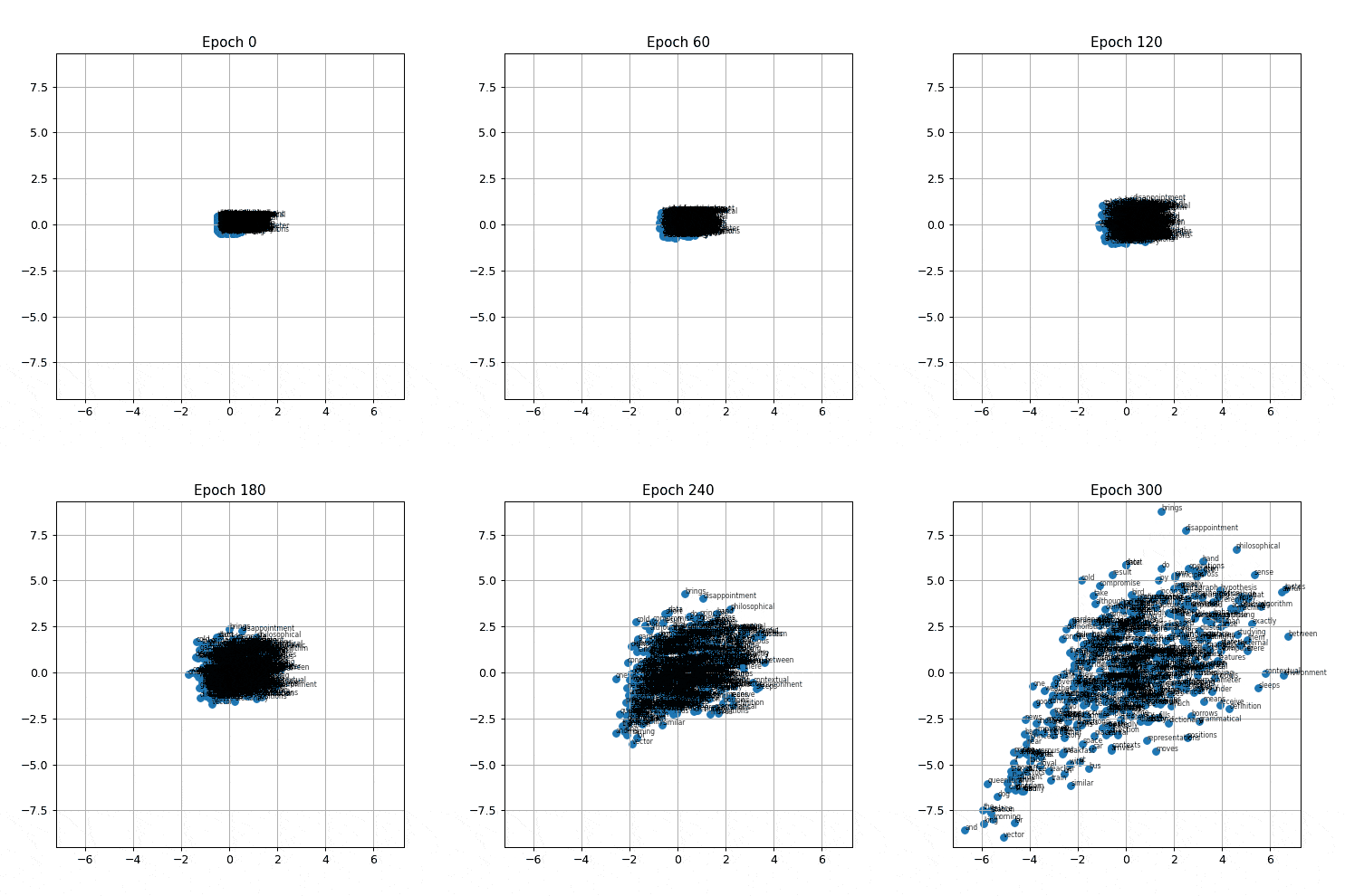
Running it in the browser
The simulator below is identical to the one in §4.6, extended with a single new slider for \(K\), the number of negatives drawn per observed pair. Setting it to \(0\) reproduces the collapse from the previous section; setting it to \(1\) or higher activates the repulsion.
It is important to note that with the repulsion mechanism, the simulation may be wobbly, but this is expected. As the vectors repel each other, the distance between them increases, causing the viewport to slowly, or in most cases rapidly, depending on the other parameter values, expand as well.
Two effects are worth watching as you play with the slider. First, at \(K = 0\) you recover the pure collapse from §4.6: the mean pairwise distance decays toward zero and every vector ends up near the origin. Second, at \(K = 1\) the collapse is gone, the mean pairwise distance stops falling and the vector space shows better semantic clusters instead of piling into a single point.

One honest note is worth making here, not only about this figure but about embedding visualisations in general. As far as I have researched, almost every scatter plot of word vectors you encounter in research papers, blog posts or lecture slides, uses the same system: a curated handful of words, often coloured by semantic category, is highlighted while the rest are muted or left out entirely.
With this system there is however, a slight inconvenience. The repulsion rule has no off-switch: it pushes two vectors apart regardless of how far apart they already are. So over many epochs, the values of the vectors grow without stopping. At a learning rate of \(0.001\), the effect is severe enough that the printed vectors scale up to 2000. At a higher learning rate, or with many more repulsions, it blows up immensely, up to \(10^{80}\), which almost amounts to the number of atoms in the observable universe.
Another interesting observation is that, words that are already on opposite sides of the space still get pushed further if one is sampled as a negative for the other. This also results in the viewport expanding as the distance keeps growing. Numerically this shows up as the mean vector norm drifting upward at \(K \ge 1\) rather than settling. Interestingly enough, we can observe this geometrically as well: the clusters still form correctly, but over time they stretch to be elongated, almost similar to a linear function instead of spreading out more evenly into compact groups. The system has stopped collapsing, but it has not found no stopping point.
Below is a simulation run that showcases this:
Simulation run that showcases the repulsion as well as the long elongated form.


So we need to fix these inconveniences first. We have to introduce a margin: a distance threshold past which two vectors are considered already far enough apart and the push simply turns off. This is the off-switch for our repulsion that has been missing. Once a pair is past the margin, the update reduces to zero and stays there. The geometry remains Euclidean throughout, building directly on the pull rule we have been using since the simplified learning. Afterwards we need to fix the sampling side by drawing negatives proportional to how often each word actually occurs, so frequent words like the stop being undercorrected and rare words stop being overpushed. Together those two pieces give us a working from-scratch contrastive embedding algorithm. The famous word2vec algorithm uses the same general structure with a different choice of update rule (dot product plus sigmoid instead of distance plus margin).
The Distance Margin
The repulsion works but does not know when to stop. Once two vectors are sampled as a negative pair, the push moves them apart regardless of how far apart they already were and over many epochs this explodes into massive distances. We need a way for the algorithm to say this pair is already far enough apart, leave it alone.
A simple idea: stop pushing when far enough
Pick a distance \(m\), called the margin. Think of it as a "personal space" radius: two word vectors are considered far enough apart whenever the distance between them is at least \(m\). Any closer than that and the push activates. Any further apart and the push does nothing. That single threshold gives us the off-switch we have been missing.
Concretely, when the algorithm samples a negative pair \((v_c, v_{\text{neg}})\), it now does three things:
1. Measure the current distance between the two vectors: \(d = \lVert v_c - v_{\text{neg}} \rVert\).
2. If \(d \ge m\), do nothing. The pair is already past the margin. This is the off-switch.
3. If \(d < m\), push the two vectors apart, with the push scaled by how far below the margin the pair currently is.
The new push rule
When \(d < m\), we update each vector by a small step in the direction that moves them apart, scaled by the factor \((m - d)/d\):
$$ v_c \leftarrow v_c + \eta \cdot \frac{m - d}{d} \cdot (v_c - v_{\text{neg}}) $$
and symmetrically for \(v_{\text{neg}}\) in the opposite direction. The factor \((m - d)/d\) is what gives the algorithm its sense of urgency:
When \(d\) is small (the pair is close together and badly placed), \((m - d)/d\) is large, so the push is strong.
When \(d\) is close to \(m\) (the pair is almost at the threshold), \((m - d)/d\) is near zero, so the push fades to nothing.
When \(d \ge m\) (the pair is past the threshold), there is no update at all.
The push therefore tapers smoothly as the pair approaches the margin, rather than slamming into a wall. By the time the pair reaches \(m\), the algorithm has gracefully run out of things to do.
The implementation in code is a small extension of the §4.7 train_on_negative: compute
the distance, check the distance, apply the scaled push if needed. This is added inside embedding_model.py.
def train_on_negative_margin(self, center_word, negative_word,
                             margin, learning_rate=0.01):
    center_vector = self.embeddings[center_word]
    negative_vector = self.embeddings[negative_word]

    # Compute the difference vector and its Euclidean length
    diff = [c_value - n_value for c_value, n_value in zip(center_vector, negative_vector)]
    distance = math.sqrt(sum(d * d for d in diff))

    # Off-switch: vectors already at least `margin` apart -> no update
    if distance >= margin:
        return

    # Protects against 0 divison
    if distance < 1e-12:
        return

    # Push apart along (center - negative) / distance, scaled by how far below the margin the pair currently is
    scale = (margin - distance) / distance
    for i in range(self.embedding_dim):
        # Push both the center vector and the sampled negative vector apart
        # moves "outward" along diff
        center_vector[i] += learning_rate * scale * diff[i]
        # moves "outward" along -diff
        negative_vector[i] -= learning_rate * scale * diff[i]
Example:
To make the off-switch concrete, imagine two 1D vectors \(v_c = 0.4\) and \(v_{\text{neg}} = 0.7\), with margin \(m = 1.0\) and learning rate \(\eta = 0.1\).
The distance is \(d = 0.3\), which is below the margin, so the push is active. The scale factor is \((m - d)/d = 0.7/0.3 \approx 2.33\). The update displaces \(v_c\) by \(\eta \cdot \text{scale} \cdot (v_c - v_{\text{neg}}) = 0.1 \cdot 2.33 \cdot (-0.3) \approx -0.07\). After the step, \(v_c \approx 0.33\) and \(v_{\text{neg}} \approx 0.77\), giving a new distance of about \(0.44\) which closer to the margin but not yet there.
Now imagine the same pair but at distance \(d = 1.5\), already past the margin. The off-switch fires and the function returns no update. The pair stays exactly where it was. Without this margin, the same pair would have received a further push.
Margin training loop integration
The §4.5 / §4.7 training loop carries over almost unchanged. We add a MARGIN
constant and call the new method instead of the old train_on_negative:
EPOCHS = 300
LEARNING_RATE = 0.001
NEGATIVES_PER_PAIR = 1
MARGIN = 1.0

vocab_size = len(word_to_id)

def sample_negative(center_id):
    while True:
        neg = random.randrange(vocab_size)
        if neg != center_id:
            return neg

for epoch in range(1, EPOCHS + 1):
    random.shuffle(pairs)
    for center, context in pairs:
        model.train_on_pair(center, context, learning_rate=LEARNING_RATE)
        for _ in range(NEGATIVES_PER_PAIR):
            negative = sample_negative(center)
            model.train_on_negative_margin(center, negative, MARGIN, learning_rate=LEARNING_RATE)
Running it in the browser
The simulator below is identical to the one in §4.7, with one new slider added: the margin \(m\). Setting \(m\) to a small value brings the off-switch on aggressively (almost every pair becomes "far enough" almost immediately, so very little pushing happens). Setting \(m\) to a large value approximates the §4.7 behaviour, since vectors never reach the threshold and the push acts as if it were unbounded. The default value \(m = 1.0\) is a reasonable middle ground for the current corpus and learning rate.
Margin observations
While running this I observed 3 things:
First and most importantly, the mean vector norm is now bounded. Compared to §4.7, where the norm drifted upward without limit, here it slowly becomes constant to roughly the size of the margin.
Second, the off-switch is observably active during training. As epochs go by, more and more pairs end up close at distance \(\ge m\). The number of actual updates per epoch shrinks and Training reaches a point where most negative samples are not pushed away, so the geometry settles.
Third, the geometry is more uniformly distributed than the cluster structure we saw briefly in §4.6 or §4.7. Every word, frequent or rare, ends up roughly equidistant from every other word, bounded by the margin.

Fourth, the clusters that do form are not always the ones a human reader would expect. The screenshot below is a typical run of the in-browser simulator:

While analysing this picture optically to evaluate the clusters I said 'HUH?'. Why is dog so close to prince and princess rather than over with cat and pets? And why are prince and princess not pulled up toward the royalty cluster around king, queen, kingdom? The geometry feels semantically wrong.
Then I realised that this does indeed make sense, with the corpus that we have. The algorithm only knows what words sit next to each other in the corpus. The sentences responsible for the geometry above are:
"the king rules the kingdom. the queen rules the kingdom."
"the prince and the princess live in the palace."
"the dog and the cat are pets in the house."
Prince and princess share the, and, plus they directly co-occur in the same sentence. Dog and cat share the, and, plus they directly co-occur in the same sentence. Both groups follow the same structural pattern: "the X and the Y", with X and Y sitting two positions away from and. From the algorithm's perspective, and is acting as a shared anchor pulling all four words prince, princess, dog, cat towards a common region.
King and queen are not in any "and" sentence in this corpus. They appear in "the king rules the kingdom", which has no and. So they cluster around rules and kingdom instead and they have no word anchor pulling them toward prince or princess. The royal connection between king and prince would not exist in this small corpus. In a much more richer corpus the royal connection will be shown.
Frequency-Biased Sampling
We could stop here since this already produces good embeddings. But after some more research and thought I decided that it was worth finetuning this even further.
Right now rare words still get pushed apart from random partners just as often as common ones do. Their final positions end up being shaped more by repulsion than by the few real attractions they take part in. Looking back at the preprocessing step, we built a vocabulary where every word is assigned a number, but that number is just an identifier and does not say anything about how often the word appears in the corpus. So when the sampler currently picks a random word from the vocabulary, a very common word like the has exactly the same chance of being picked as a really rare word that only appears once. This is something we can improve to make the embeddings better.
We can fix this by improving the sampler: instead of picking negative words completely at random, we pick them in proportion to how often each word actually appears in the corpus.
The problem with our current uniform sampling
On the 459-word corpus the project has been training on, the most common word the appears \(164\) times across \(1{,}788\) total tokens, so around \(9\%\) of all word occurrences. The rarest words appear only once. Under the current negative sampling, every word in the vocabulary has the same \(1/459 \approx 0.22\%\) chance of being picked as a negative, regardless of how often it actually shows up in the text.
This is a bit of an imbalance. As a real partner in a training pair, the shows up about \(9\%\) of the time. As a uniform-random negative, it shows up about \(0.22\%\) of the time. So the is being asked to do attraction work at roughly \(40\) times the rate it is being asked to do repulsion work. This also meas that a word that appears once in the corpus is asked to do attraction work less than \(0.06\%\) of the time, but is asked to do repulsion work at \(0.22\%\) of the time, which is about \(4\) times more repulsion than attraction.
The fix: sample by frequency
The fix is to sample negative words proportionally to how often they appear, not uniformly.
For the the example, under uniform sampling we have \(P(\text{the}) = 1/459 \approx 0.22\%\). Under pure frequency-proportional sampling, \(P(\text{the}) = 164/1788 \approx 9.2\%\). The frequent word is now being sampled as a negative at exactly the rate it appears in the corpus.
But pure frequency can be a bit too aggressive. The word the is so common that under pure frequency it would be the negative target almost \(1\) in \(10\) times. That means roughly half of every reasonable batch of negative samples would just be the paired with whatever the current center happens to be. The model would spend most of its repulsion budget pushing every word away from the, with not much left over for everything else. Mikolov et al. explained in a follow-up paper to the original word2vec called Distributed Representations of Words and Phrases and their Compositionality, smoothed the distribution by raising each count to a fractional power:
$$ P(w \mid \text{negative}) \;\propto\; \mathrm{count}(w)^{0.75} $$
The effect is that frequent words are still sampled more often than rare ones, but the gap between them is dampened. For the under this smoothing, \(P(\text{the}) \approx 4.2\%\). Still about \(20\) times more often than uniform, but only half as often as pure frequency.
A note on the \(0.75\): this is an empirical constant, not a derived one. Inside that paper, the team tried different exponents on their tasks and \(0.75\) (or \(3/4\)) worked best. It is a parameter to be played with, not a principle. On a different corpus or with a different downstream task the optimal value might be different, \(0.5\) or \(0.9\), but in practice according to the paper, \(0.75\) has held up well enough across a wide range of settings.

Implementing the sampler
The sampler is a small standalone class. It builds the cumulative distribution once at construction time, then samples in \(O(\log V)\) by picking a random number in \([0, \text{total})\) and binary-searching where it falls in the cumulative array.
import bisect
import random

class UnigramSampler:
    def __init__(self, word_counts, exponent=0.75):
        self.word_ids = sorted(word_counts.keys())
        self.weights = [word_counts[wid] ** exponent for wid in self.word_ids]

        # Cumulative distribution: cumulative[i] = sum of weights[0..i].
        self.cumulative = []
        running = 0.0
        for w in self.weights:
            running += w
            self.cumulative.append(running)
        self.total = running

    def sample(self, exclude_id=None):
        while True:
            x = random.uniform(0.0, self.total)
            idx = bisect.bisect_right(self.cumulative, x)
            if idx >= len(self.word_ids):
                idx = len(self.word_ids) - 1
            sampled = self.word_ids[idx]
            if sampled != exclude_id:
                return sampled
Walking through the algorithm: at construction time, we compute
\(\mathrm{count}(w)^{0.75}\) for every word, then build a running-sum array
(cumulative) where the last entry is the total weight. To sample, we pick a
uniform random number \(x\) in \([0, \text{total})\) and binary-search for the first index
whose cumulative sum is greater than \(x\). That index corresponds to the sampled word.
If it equals the excluded id (typically the current center word), we reroll. The reroll
terminates almost immediately on any reasonable vocabulary because the excluded word's
probability is small.
In the training loop, the change is one line: build the sampler from the corpus counts, then
replace the uniform random.randrange with sampler.sample().
EPOCHS = 300
LEARNING_RATE = 0.001
NEGATIVES_PER_PAIR = 1
MARGIN = 1.0
EXPONENT = 0.75

# Build the sampler once, before the training loop
sampler = UnigramSampler(word_counts, exponent=EXPONENT)

for epoch in range(1, EPOCHS + 1):
    random.shuffle(pairs)
    for center, context in pairs:
        model.train_on_pair(center, context, learning_rate=LEARNING_RATE)
        for _ in range(NEGATIVES_PER_PAIR):
            negative = sampler.sample(exclude_id=center)   # <-- the only line that changed
            model.train_on_negative_margin(
                center, negative, MARGIN,
                learning_rate=LEARNING_RATE,
            )
That is the entire algorithmic change. Everything else, namely the pull rule from §4.5, the margin-gated push from §4.8, and the rest of the pipeline, stays exactly the same.
Running it in the browser
The simulator below is the §4.8 simulator with one new control added: an exponent slider. At the upper end (\(\text{exponent} = 1.0\)) the sampler is pure frequency-proportional. At the lower end (\(\text{exponent} = 0.25\)) the distribution is heavily smoothed and gets close to uniform.
One thing to keep in mind about the in-browser corpus: it has \(38\) words, most appearing only \(1\) to \(3\) times each, so the difference between exponents is subtle to watch live. The Python script on the \(459\)-word corpus shows the effect more clearly, and the cosine evaluation in the next subsection shows it best.
Observations on Frequency-Biased Sampling
First, the embedding geometry barely shows any difference. The side-by-side scatter below puts the §4.8 final state next to the §4.9 final state. The two clouds look very similar at this scale and on a corpus this size. Mean vector norm and mean pairwise distance are also nearly identical between the two when the embedding dimension is high enough to give the algorithm room to work. The §4.9 final state looks a bit more compact though.

Second, and most importantly, the actual quality of the trained vectors improves. The right way to measure that is cosine similarity on representative word pairs, not summary statistics over the whole cloud.
The table below summarises the cosine similarity of ten representative pairs under both samplers. The first five pairs are word pairs that should end up similar in a good embedding; the bottom five pairs should end up unrelated. Green deltas mark improvements (higher cosine for similar pairs, lower cosine for unrelated ones) while red marks regressions, and grey is essentially flat.
| Word pair | (§4.8) | (§4.9) | Δ | Notes |
|---|---|---|---|---|
| Similar pairs - want high cosine | ||||
| king/queen | +0.50 | +0.59 | +0.09 | clear improvement |
| dog/cat | +0.40 | +0.56 | +0.16 | substantial improvement |
| bus/train | +0.84 | +0.87 | +0.03 | small improvement |
| coffee/tea | +0.77 | +0.80 | +0.03 | small improvement |
| prince/princess | +0.49 | +0.47 | −0.02 | essentially flat |
| Unrelated pairs - want low cosine | ||||
| library/tea | +0.23 | +0.03 | −0.20 | substantial improvement |
| teacher/dog | +0.25 | +0.20 | −0.05 | small improvement |
| dog/morning | +0.20 | +0.15 | −0.05 | small improvement |
| king/coffee | +0.27 | +0.24 | −0.03 | small improvement |
| queen/breakfast | −0.02 | +0.08 | +0.10 | single regression |
The "similarity gap", which is the average cosine of related pairs minus the average cosine of unrelated pairs, widens by about \(0.10\) under §4.9. That is a real, consistent shift on \(8\) of \(10\) representative pairs, and it is exactly the kind of improvement frequency-biased sampling is supposed to produce. Rare content words get less random repulsion, so their final positions are driven more by their few real attractions and less by noise.
Another note on the Frequency-Biased Sampling: The improvement above is modest, partly because the corpus is small (\(459\) words versus the billions most other state of the art word-embeddings were originally trained on) and partly because the rare-word problem is much more severe on real text, where the long tail of low-frequency words is far heavier. The qualitative claim that frequency-biased sampling produces better cosine similarity on rare-word pairs would still hold on a much larger corpus, and the magnitude of the effect would be much larger too.
With this swap in place, the project now has a working from-scratch contrastive word-embedding algorithm. It pulls related words together (§4.5), it pushes random pairs apart with an off-switch when they reach the margin (§4.8), and it samples those random pairs proportional to how often each word actually appears in the corpus (§4.9). Three rules, one new idea per section, applied to a corpus of arbitrary size.
For readers who have followed the project all the way through, you might notice that what we have been doing is essentially a divide-and-conquer approach. I did not set out to apply it deliberately, but looking back at the chapters now, that is exactly what happened. The larger task of building word embeddings was broken into a sequence of smaller sub-problems: representing words as vectors, pulling related ones closer together, pushing random pairs apart, adding an off-switch so the pushing did not run away and then finally biasing the sampler so frequent and rare words were treated proportionally to how often they appear. Each section tackled one piece, and the pieces combined cleanly into a working algorithm. I found that satisfying to notice only in hindsight.
Evaluating the Embeddings
The previous chapter was all about building the system and explaining individual parts that make it. This chapter is about putting it to use. The previous experiments, all ran on a more smaller and compact corpus designed to make the geometry visible in 2D. To be precise, the corpus inside the github repository, which was self-written and used in the plotting illustrations, contained around 1800 words and 106 sentences. The one used inside the browser for the simulation runs has around 10 sentences. We now need to test the algorithm on a bigger corpus, use more dimensions and find a way to measure quality of the embeddings.
Nearest Neighbours
For this evaluation we train on the
Brown corpus,
a 1.1 million token collection of American English text from 1961 that NLTK ships out of
the box.The training script, which can be found inside the github repository, is train_brown.py and it is configured
with 10,000 vocabulary words, 50-dimensional embeddings, 5 negative samples per pair,
the §4.9 frequency-biased sampler at
exponent \(0.75\), and 10 training epochs. The training time took on my own MacBook M5 Pro arond 50s per epoch, so around 8 minutes in total.
With the corpus and training now out of the way, the natural next question is: given a trained model, what
words come out as the nearest neighbours of king, or
coffee, or monday? This is the standard
cosine-similarity query. Take a target word's vector, compute the cosine between it and
every other vector in the vocabulary, and return the top \(K\) most similar.
Querying is done with nearest_neighbours.py, which loads the
saved embeddings and prints the top-\(K\) cosine matches for any word you ask about.
Three clean clusters
Three queries produce textbook-quality results. The kind of output that makes the algorithm look obviously right at a glance.
| Query | Top 5 nearest neighbours (cosine similarity) |
|---|---|
| monday | wednesday +0.93, sunday +0.90, tuesday +0.89, saturday +0.89, friday +0.86 |
| january | june +0.90, july +0.87, february +0.82, april +0.82, december +0.79 |
| bread | butter +0.85, salad +0.84, cheese +0.84, cream +0.81, soup +0.81 |
Days of the week, months, and baking ingredients each form sharp clusters where every neighbour comes from the same semantic category. The model has correctly identified that words appearing in similar syntactic and semantic roles end up near each other in the embedding space.
Pairwise cosine checks
For specific word pairs, the cosine similarity is a single number we can read off directly. Four representative pairs:
| Word pair | Cosine | Notes |
|---|---|---|
| man/woman | +0.80 | strong gender pair |
| dog/cat | +0.57 | moderate same-category |
| king/queen | +0.51 | moderate, corpus-shaped |
| dog/january | −0.01 | correctly unrelated |
The first three pairs are positive and roughly tracking semantic similarity. The fourth is near zero, which is exactly what we want from an algorithm that does not manufacture similarity between unrelated words. The king/queen cosine is lower than man/woman, which feels counterintuitive at first but reflects a real property of the Brown corpus: king-contexts are dominated by named historical kings (Arthur, James, Henry) rather than the abstract concept of royalty. The model learns what is near a word, not what the word means in the abstract.
Honest limitations
Not every query produces a clean cluster. Querying dog and cat surfaces each other near the top, but most of the rest of their neighbours are noise: wreath, charcoal, sheet, contest. Brown is not a pet-heavy corpus, so the model never sees enough sentences about household pets to anchor a tight cluster. With a larger or more pet-relevant corpus this would resolve.
One broader limitation worth naming: embeddings reflect their training data, including parts of it we would not endorse. Brown contains text from 1961 with cultural artefacts and slurs that appear naturally in its literary and quoted-speech categories. A distributional model trained on Brown will surface these in its nearest-neighbour results, because the model has no way to filter them out. This is not a bug in the algorithm. It is a consequence of training on real text without any preprocessing step for offensive language. For a production system one would clean the corpus or filter the model's outputs.
With the nearest-neighbour structure confirmed, the next question is what the embedding space looks like geometrically. §5.2 takes a curated subset of words, projects the 50-dimensional embeddings down to 2D with PCA, and plots the result.
Embedding Space Visualization
Cosine queries tell us about individual word pairs but they cannot show us the overall shape of the embedding space. For that we need to look at the full geometry, which is a problem because the geometry lives in 50 dimensions and we can only draw in two. The standard tool for compressing high-dimensional data down to two dimensions for plotting is Principal Component Analysis, usually shortened to PCA. The mathematical idea: find the two directions in the original 50-dimensional space along which the points are most spread out, and project everything onto those two directions. The result is the closest 2D approximation of the original cloud, in a precise sense of "closest" that PCA defines.
For this visualization we pick a curated list of around 70 words organised into 10
semantic categories (days of the week, months, time of day, food, family, body parts,
numbers, colours, nature, US politics, plus ten more groups). Each point in the viewer
below is one word, positioned in 3D PCA space and coloured by its category. Hover a
point with the mouse to reveal the word and its category. Click-and-drag to rotate, use
the scroll wheel to zoom, and right-click-drag (or two-finger drag on a trackpad) to
pan. The script is visualize_embeddings.py in the project; PCA is
implemented from scratch in five lines using NumPy's SVD.
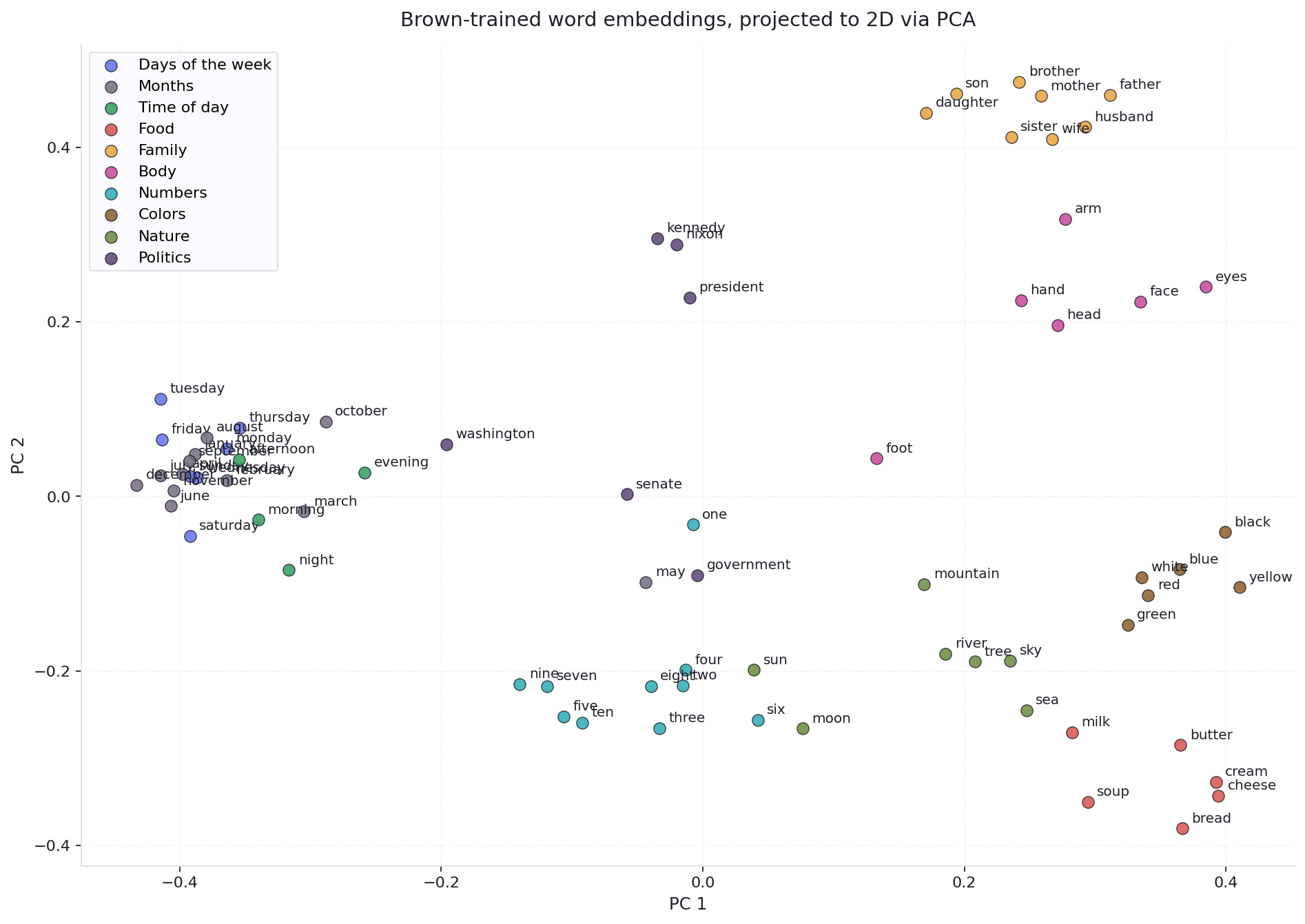
A few patterns stand out. Days of the week and months cluster tightly on the left side of the plot, sitting almost on top of each other. Time-of-day terms (morning, evening, night) sit immediately next to them, which makes sense because time in general co-occurs with similar surrounding words.
Family terms form a clean cluster in the upper right (father, mother, brother, sister, son, daughter, husband, wife), and the body-part cluster (head, hand, face, eyes) sits adjacent to it. The model mapped them correctly as adjacent regions.
Numbers form their own cluster in the lower middle (one until ten). Nature words (sea, mountain, river, sky, sun, moon, tree) are more spread out, occupying the middle and right of the plot. Politics terms (president, kennedy, nixon, washington) sit roughly in the centre, with some scatter.
The food group also sits nicely together. One observation that I made, is that the color white seems to drift off a bit further.Red, black, yellow hang together on the right, but white is sligthy different, which is the model most likely picking up on "white house" appearing as a phrase in Brown's political coverage.
Two caveats worth naming
First, this is still a coloured cherry-picked visualization. I decided the word list. I decided the categories. I decided the colour mapping. Showing the same 70 words without colour would look like a mist cloud of dots and the everyone would have a much harder time seeing the structure.
Second, projecting from 50 dimensions to 2 throws away most of the information. The first two principal components typically capture a small fraction of the total variance in word embeddings (around \(15\%\) to \(25\%\) on a corpus this size). What you see in this plot is the 'shadow' of the embedding space, not the full embedding space itself. Two clusters that look adjacent in 2D might actually be separated along a dimension that did not survive the projection; two clusters that look distant might be much closer if you measured in the full 50D. Cosine similarity in 50D is the more accurate way to measure the overall quality quality.
Where this leaves us
I started this whole project with one question: how do you teach a computer that coffee and tea are related, when neither is anything more than a sequence of letters? Five chapters later, we built a system that can understand semantic relationship between words. The overall architecture consits of: Build vectors, pull related ones together, push unrelated ones apart with a margin, sample those negatives proportional to frequency, train on real text, then ask the trained model what it thinks. The model we built is a simple variant of word2vec. It uses Euclidean distance instead of dot products for training, a margin instead of a sigmoid, a single embedding matrix instead of two, and no subsampling of frequent words.
That said, we successfuly made a word-embedding system from scratch. Days of the week cluster, months cluster, family terms cluster and other semantic groups are clearly visible. The cosine similarity tests that we ran for validation also showed us that the embedding space captured meaningful relatinships between these words.
Overall, working on this project was really fun. I remember when I started it, I was deeply intrigued by the idea of diving into Natural Language Processing. It always baffled me to understand how, mathematically speaking, you could ever possibly capture the semantic meaning of words and allow a computer to store that meaning, which is the embedding space. There have been many lessons learned, and I can confidently say that this topic has deepened my understanding of NLP. I remember reading papers, not only technical ones but also from the linguistics department. Some of them dated back even 30 years, long before I was born, explaining how the meaning of a language can be understood just by looking at words and their neighbors. If you have reached this section, then thank you for your time and for reading one of my projects. I have spent many hours documenting and working on this project, it has been a great journey. Lastly, I want to thank my supervisor Dr. Christian Steineder for giving me the opportunity to work on a project that I truly enjoyed, and for providing guidance along the way.
References
- Z. Harris, “Distributional Structure,” Word, vol. 10, no. 2–3, pp. 146–162, 1954. [Online]. Available: [PDF]
- M. Sahlgren, “The Distributional Hypothesis,” Italian Journal of Linguistics, vol. 20, no. 1, pp. 33–53, 2008. [Online]. Available: [PDF]
- J. R. Firth, A Synopsis of Linguistic Theory, 1930–1955. Oxford, U.K.: Blackwell, 1957.
- S. Deerwester, S. T. Dumais, G. W. Furnas, T. K. Landauer, and R. Harshman, “Indexing by Latent Semantic Analysis,” Journal of the American Society for Information Science, vol. 41, no. 6, pp. 391–407, 1990. [PDF]
- T. Mikolov, K. Chen, G. Corrado, J. Dean, “Efficient Estimation of Word Representations in Vector Space”, arXiv preprint arXiv:1301.3781, 2013. [Online]. Available: [PDF]
- T. Mikolov, I. Sutskever, K. Chen, G. Corrado, J. Dean, “Distributed Representations of Words and Phrases and their Compositionality”, Advances in Neural Information Processing Systems, vol. 26, 2013. arXiv preprint arXiv:1310.4546. [Online]. Available: [PDF]
- J. Pennington, R. Socher, and C. Manning, “GloVe: Global Vectors for Word Representation,” Proceedings of the 2014 Conference on Empirical Methods in Natural Language Processing (EMNLP), pp. 1532–1543, 2014. [Online]. Available: [PDF]